Morpheus

This is an old revision of the document!

Reaction-diffusion models

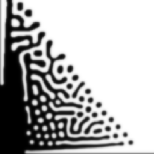
Domains: Reaction-diffusion in irregular domains

Spot pattern in Gierer-Meinhardt model with irregular domain

Introduction

A 2D activator-inhibitor model (Meinhardt and Gierer, 1972), solved in a irregular domain that is load from file.

Model description

This model uses an irregular Domain with constant boundary conditions. The domain is loaded from a TIFF image. See Space/Lattice/Domain.

Model

Note: This model requires the external file domain.tif (download domain.tif).

h ActivatorInhibitor_Domain.xml |h

extern>http://imc.zih.tu-dresden.de/morpheus/examples/PDE/ActivatorInhibitor_Domain.xml

In Morpheus GUI: Examples → PDE → ActivatorInhibitor_Domain.xml

Spatial parameter sweep: Turing patterns

Spots and stripes appear under various conditions in linear Turing model

Introduction

This model shows the pattern formation abilities of Turing's linear activator-inhibitor model (Miyazawa et al., 2010). It shows how to vary parameters as a function of space.

Model description

Instead of fixed parameters defined as Constants, this model uses Functions for two parameters. The parameters C (activator production) and A (rate of auto-activation) as defined as Function of space and varied over the X- and Y-axes respectively. This requires the definition of a SpaceSymbol that can be used in expressions.

The results show the appearance of white spots (left), black spots (right) and labyrinthine patterns (middle).

Model

h TuringPatterns.xml |h

extern>http://imc.zih.tu-dresden.de/morpheus/examples/PDE/TuringPatterns.xml

In Morpheus GUI: Examples → PDE → TuringPatterns.xml

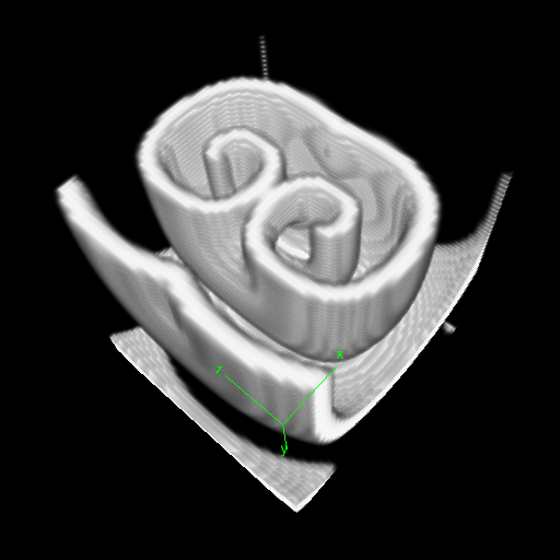
3D reaction-diffusion: Excitable Media

Scroll wave appear in Barkley model of excitable media in 3D

Introduction

This example uses the Barkley model of excitable media, similar to the Fitzhugh-Nagumo model to show how to model and visualize reaction-diffusion models in 3D.

Model description

This model defines a 3D cubic Lattice with noflux BoundaryConditions. Two Layers are defined for the two species: 'u' is the signal, and 'v' the refractoriness. As in the examples above, the DiffEqn as specified in the System in PDE. Nothing strange here.

To visualize the resulting scrolling waves in 3D, the TiffPlotter is used. This Analysis plugin writes TIFF image stacks that cam be opened by image analysis software such as Fiji/ImageJ. To import Morpheus TIFF images into Fiji, macros scripts are available that help you to create 3D (xyz), 4D (xyzt) or even 5D (xyzct) images and movies of your simulations.

Although unable to plot 3D, the GnuPlotter can still be helpful to plot a 2D slice. See Analysis/Gnuplotter/PDE/slice.

Model

h ExcitableMedium_3D.xml |h

extern>http://imc.zih.tu-dresden.de/morpheus/examples/PDE/ExcitableMedium_3D.xml

In Morpheus GUI: Examples → PDE → ExcitableMedium_3D.xml

Things to try

Import resulting sequence of TIFF images in ImageJ or Fiji, and create 4D movie using ImageJ's 3D plugin:
1. Open u_v.tif in ImageJ: File → Open.
2. Create hyperstack: Image → Hyperstack → Convert to Hyperstack. Channels ( c ): 2, Slices (z): 50, Frames (t): 51, Display Mode: Composite.
3. Display in 4D: Plugins → 3D Viewer. Use default parameters. Press OK.