
This is an old revision of the document!
Frequently asked questions
General
More information
For more information, refer to the user manual.
What it cannot do
See the necessarily incomplete list of limitations.
Morpheus is a self-contained application. Internally, it consists of two stand-alone executables:
morpheus: the simulatormorpheus-gui: the graphical user interface (GUI)
The communication between these stand-alone applications is through XML and XSD files:
- The GUI reads an XML Schema description (XSD) file that specifies rules for valid XML models.
- The GUI start a simulation job by executing
morpheuswith a generated XML model as argument.
Note that both executable can also be used as stand-alone programs. The simulator morpheus can also be used as stand-alone program from the command line. And morpheus-gui may be used to control remote computing resources.
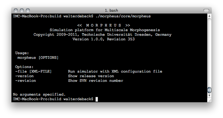
morpheus simulator from the command line interface. Source
The source code publicly available at GitLab
Building from source
Information on building Morpheus from source can be found here.
User forum
Use the Morpheus user forum to get support from developers and other users.
User manual
The user manual is the primary source of information on usage of Morpheus.
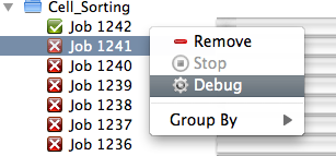
Debug mode
Run your model in debug mode by select the crashed job in the Job Queue, then right-click and choose Debug. This requires that you have gdb (Gnu Debugger) installed.
Debug mode, and send us the log file gdb.log.Morpheus is developed by Jörn Starruß and Walter de Back at the IMC group headed by prof. Andreas Deutsch.
We are part of the Center for High Performance Computing at the Technische Universität Dresden, Germany.
Modeling
Use an example
The easiest way to start to create your own models, is to browse the Examples and use them as templates. The examples can be found under File→Examples.
Start from scratch
To start from scratch, use File→New. This will generate a minimal valid model. Then, check out how to edit models.
Required and optional model items
Each valid MorpheusModel specifies the following required items:
Description: Title and description of modelSpace: Lattice size, structure, length scale and boundary conditionsTime: Simulation duration, checkpointing, time scale, and random seed.
And may be extended with the following optional items:
CellTypes: Definition of cell types, their properties and behaviorsCPM: Specific parameters for cellular Potts modelPDE: Specification of reaction-diffusion systemCellPopulations: Specification of cell population and spatial layout
And can be analyzed using the following optional items:
Analysis: Data, analysis and visualization toolsParamSweep: Batch processing tool (in GUI)
Types of Boundary Conditions
Morpheus provides three types of boundary conditions.
| Types of BoundaryConditions | ||
|---|---|---|
| Name | Synonym | Meaning |
| Periodic | Wrap-around | Border states are mapped to states at opposite border. |
| Constant | Dirichlet | Border states have specified constant values. |
| Noflux | Neumann | Derivative at border is zero. |
These can be specified in Space → Lattice → BoundaryConditions. These define the structure of the boundaries.
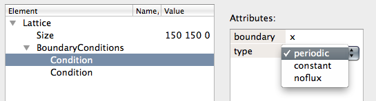
Space → Lattice → BoundaryConditions.
Note that there are six boundaries (x, -x, y, -y, z, -z). All need to be specified, expect when periodic boundaries are used (in which case x=-x, y=-y, z=-z).
Constant boundary condition
To define constant boundaries, select constant in Space → Lattice → BoundaryConditions.
To specify the values the constant boundaries should take, we distinguish between reaction-diffusion models (PDE) and cell-based models.
Reaction-diffusion models (PDE)
When using constant boundary conditions, values used at the boundary of a reaction-diffusion model can be specified in PDE → Layer → BoundaryConditions. Assuming nonzero diffusion, this causes a constant influx (or efflux) from (at) that boundary. The default value is $0.0$.
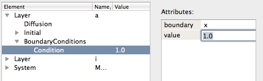
PDE → Layer → BoundaryConditions. Cell-based models
A particular medium cell type can be specified at constant boundaries. First, define a cell type of type medium under CellTypes. To specify this at the boundary of a cell-based model with constant boundary conditions, use CPM → BoundaryConditions.
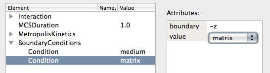
CPM → BoundaryConditions.
To specify initial conditions, we distinguish between reaction-diffusion models (PDE) and cell-based models.
Reaction-diffusion models (PDE)
To set an initial condition for a species in the reaction-diffusion model, specify it in PDE → Layer → Initial → InitPDEExpression → Expression.
Note that you can express the initial condition in terms of the lattice size using the symbols set in Space → Lattice → Size/symbol (here: s) and Space → SpaceSymbol (here: l).
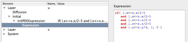
PDE using InitPDEExpression in terms of spatial symbols for lattice size.Cell-based models
Initial conditions for a Property of a CellType are specified when you define the Population of cells. Set the initial values using CellPopulations → Population → InitProperty.
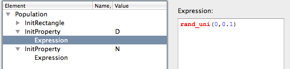
Properties using InitProperty in the Population definition. Random seed
- Mersenne Twister from C\+\+ compiler (gcc version > 4.6) or Boost library when available.
Time→RandomSeed
Reproducibility
- In simulation using multithreading (openMP), each thread gets its own random seed. Therefore, to reproduce exact results, one needs to specify the same random seed as well as the same number of threads.
Specifying time scales is important, especially in multiscale models in which dynamics occur at multiple temporal scales.
In Morpheus, we distinguish three time scales:
- Global time: defines the time frame of a simulation.
- Monte Carlo time scale: defines updating scheme of cells.
- System time scale: defines updating and dynamics of systems of (differential) equations.
Global time
Each model must specify a global time scheme under Time that runs from StartTime to StopTime. All other processes are scheduled within this time frame.
For dimensionless models, a sensible choice for the global time scheme would be from $0$ to $1$. For an example, see the cell cycle model (File → Examples → MultiScale → CellCycle).
Alternatively, for dimensional models, time units can be specified (msec, sec, min, hours, days) such that one could define the global time to run from 20 hours to 7 days. Default interpretation is 1 sec.
Monte Carlo time scale (CPM)
The time scale of cellular Potts models can be specified using CPM → MCSDuration. This defines the interval between Monte Carlo steps, in terms of global time scheme.
For example, if the global time is defined from $0 \rightarrow 1$, and MCSDuration is set unitless to $1.0\cdot10^{-2}$, a total of $100$ Monte Carlo steps will be performed during the simulation.
Alternatively, if the global time is defined with dimenions from $0$ hours to $1$ hours, and MCSDuration is set to $1.0$ sec, a total of $3600$ Monte Carlo steps will be performed during the simulation.
Note that changing the MCSDuration time scale directly affects the CPM dynamics such as cell motility and cell shape changes. In fact, it will affect all processes under CellTypes → CellType, except the processes defined within Systems.
System time scale (ODE/PDE)
To define the time scale for a System of (differential) equations, we need to distinguish between:
- Numerical updating scheme: how often the equations with the systems are evaluated.
- System dynamics: setting the time scale of ODE model dynamics, relative to the global time.
The numerical updating of a system of equations is defined in System → time-step (default=$1$), in terms if the global time scheme. This sets the accuracy of the numerical approximation (i.e. it is the $ht$ of the numerical solver), but does not affect the time scale of its dynamics.
To change the time scale of the dynamics of simulated ODE model, you can use the System → time-scaling attribute. This scales the rates of dynamics, while maintaining the accuracy (by automatically scaling the time-step). For an example, see the multi-scale cell cycle model (File → Examples → Multiscale → CellCycle).
Lattice scale
Space → NodeLength
This affects the diffusion coefficient in PDE models.
Dimensionless space is assumed, unless a unit is specified.
Types of Neighborhoods
Two types of neighborhood are used:
Space → Lattice → Neighborhood: …CPM → MetropolisKinetics → Neighborhood: …
Order and Distance
The number of neighboring nodes to include can be specified in two different units:
- Distance: All nodes ⇐ this distance are included in the neighborhood.
- Order: All nodes of this order are included in the neighborhood.
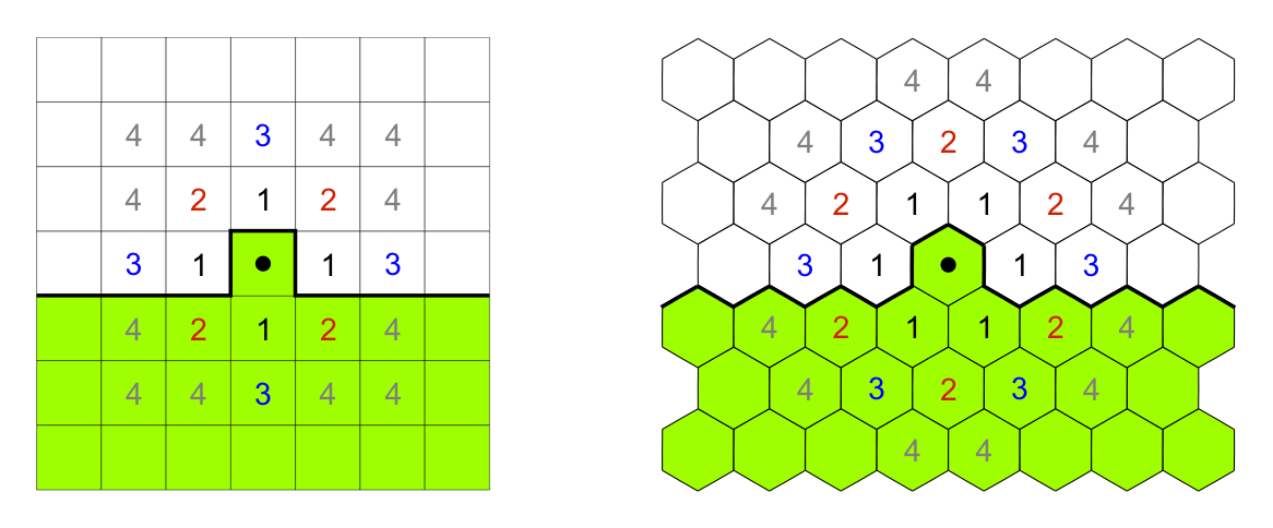
Order
The “order” of a neighborhood is a measure of neighborhood size that expands in an alternating way axially and radially.
In a square lattice:
- Order 1: 4-member, axial (von Neumann)
- Order 2: 8-member, radial (Moore)
- Order 3: 12-member, axial
- …
Both are algebraic expressions, however:
- A
Functiondefines asymbol, and it calculated whenever this symbol is used. - An
Equationchanges the value of a symbol defined elsewhere (symbol-ref) and is calculated everytime-step.
Note: if anEquationis part of aSystem, thetime-stepof theSystemoverrules the one defined by theEquationitself.
| Attribute | Evaluation | |
|---|---|---|
Function | symbol | Evaluated when symbol is used |
Equation | symbol-ref | Evaluated every time-step (default=1), set result to referred Property |
Analysis
Use the Gnuplotter. See the Examples to learn how to use it.
3D visualization
To visualize 3D simulations, Morpheus can write TIFF images stacks or VTK files.
These files can be rendered with external software, such as Fiji or Paraview.
Viewing 3D TIFF images with Fiji/ImageJ
To export 3D images as TIFF z-stacks, use the Analysis → TiffPlotter plugin.
The resulting TIFF images can be opened using the 3D Viewer in Fiji, an image processing package based on ImageJ (see Plugins → 3D Viewer).
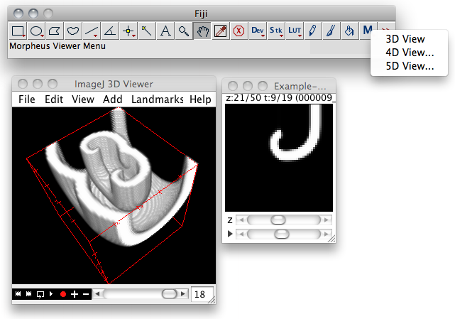
TiffPlotter for 3D, 4D or 5D visualization in Fiji.
By concatenating TIFF stacks, you can also render 4D (3D+time) or even 5D (3D+time+channels) movies.
Fiji Macros
We provide some simple Fiji macros to generate such 3D images and 4D/5D movies. To install them:
- Download morpheus_fiji_viewers.zip
- Extract contents in Fiji/macros
- Mac: Select
Applications/Fiji.app, then right-click and selectShow Package Contents. - Ubuntu: Default location is
$HOME/Fiji.app/macros
This will install a new toolset in the Fiji interface called Morpheus Viewer from which the 3D/4D/5D viewers are available.
Paraview
Paraview is an application for visualization of large 3D data sets in VTK format (download here).
Logger
Note: this plugin will be restructured in the near future.
The Logger periodically writes the values of the symbols specified in the Format to file.
Its Plot function can generate timeplots, or phase plots, depending on the columns selected for the axes. Note: these columns correspond to the column number in the generated data file (first column = 1).
HistogramLogger
HistogramLogger calculates frequency distributions and writes them to file.
Its Plot function can generate timeplots.
Parameter sweep / Batch processing
To explore the effect of a parameter on model behavior, you can set up a batch process called ParamSweep.
1. Select parameters
In the Attributes window, press right-click on a parameter and choose ParamSweep. A 'fast-forward' symbol appear indicating that this parameter is set for a parameter sweep.
Alternatively, if no Attributes windows is available (e.g. with Expression), right-click in the central window to select for ParamSweep.
Note that model parameters of any type can be explored (double, int, string, enum, etc.).
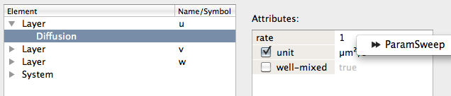
Attributes window to select parameter for ParamSweep2. Set range of values
Once you have chosen a parameter, go to the ParamSweep view (see Documents window).
Here, you can specify a range of values for each parameter.
| Syntax | Example | Generated sequence | Description |
|---|---|---|---|
| value1;value2;value3 | 1.0;1.25;4 | 1.0;1.25;4 | Sequence of values |
| string1;string2;string3 | “square”;“hexagonal” | “square”;“hexagonal” | Sequence of strings |
| min:increment:max | 0:2:10 | 0;2;4;6;8;10 | Range of values with increment |
| min:#steps:max | 0:#2:10 | 0;5;10 | Range of values with number of steps |
| min:#steps[log]:max | 0.1:#2log:10 | 0.1;1.0;10.0 | Range of values with number of steps in logarithmic scale |
The Number of Jobs that will be generated is calculated and displayed.
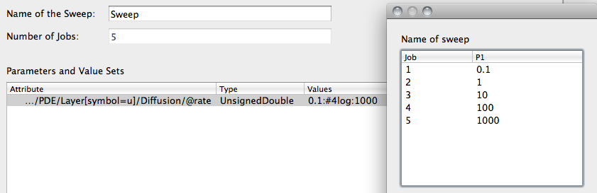
ParamSweep window and execute batch process by pressing Start.
3. Execute ParamSweep
To start a parameter sweep, press Start in the toolbar while you have the ParamSweep panel open.
Before it starts the batch process, Morpheus let's you check your jobs and parameters in a pop-up window.
Also note that batch processes can benefit from parallel computing by allowing multiple concurrent jobs, see Settings → Local → Concurrent Jobs.
Note that the parameter sweep is always run in Local mode (overrides Interactive mode).
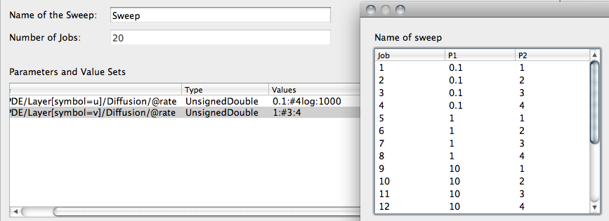
Multi-dimensional ParamSweeps
Multi-dimensional parameter sweep are generated by selecting multiple parameters for ParamSweep.
To couple multiple parameters such that they are incremented simultaneously, drag one over the other to 'pair' them.
How to post-process results of a parameter sweep?
Morpheus does not include tools for post-processing of data. Thus, analyzing results should be done using your own favorite tools.
Yet, Morpheus does supply a few features that enable you to analyze results of parameter sweeps:
- Sweep summary: file containing data on parameters and the folder in which the results are saved.
- Python scripts:
- morphMakeTable.py: generate $Latex$ table from images from a parameter sweep (using sweep summary)
- morphSweepData.py: gather data from log files from a parameter sweep (using sweep summary)
ImageTable
This option can be used to create a $Latex$ table of images from a parameter sweep. This is a simplified interface to the python script morphMakeTable.py.
Editing
Add/Remove in Document view
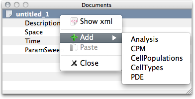
To add or remove optional model components such as PDE, CellTypes, or CellPopulation, right-click in the Documents View and choose Add or Remove.
Add/Remove in Editor view
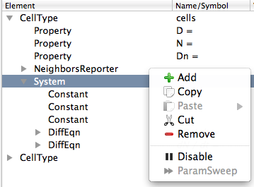
To add or remove optional plugins, right-click on the parent node and choose Add or Remove. The parent node is the place on which the new plugin should appear.
In case of Remove, you will be prompted to confirm the removal.
Save to Clipboard
To remove but save a copy on the Clipboard, choose Cut. You will not be prompted for confirmation.
Copy
To copy an item, right-click in the editor view and choose Copy. The XML snippet will be shown in the Clipboard.
Paste
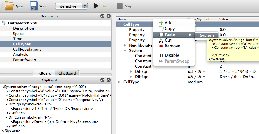
To paste an item that appears on the Clipboard, right-click in the editor view on the parent item and choose Paste. Choose an item from the drop-down list.
Note that you can copy/paste between different models.
An extract of the XML will be shown as a tooltip. This enables you to distinguish items with identical names.
Clipboard
Snippets of XML that were copied or cut are shown here. The Clipboard is shared over all models in the Documents view.
Copy/Paste between models
During model construction, it is often useful to copy/paste items between different models that appear in the Documents view. For instance, to integrate single-scale models into a multi-scale model.
This is possible, because the Clipboard is shared over all models in the Documents view.
Disable
During the model construction or testing process, it is often desirable to temporarily switch off an item of the model without removing it from the model.
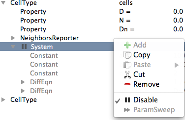
To switch off an item, right-click in the editor view and choose Disable. A 'pause' symbol appears before the node, and the item as well as its child nodes are grayed out.
Note that the item is still saved to XML, but is commented out.
Re-enable
To re-enable, do the same: right-click in the editor view and choose Disable.
Disable.Text editor
The XML files can be opened in any text editor that allow you to manually edit the model.
Command line tools
More advanced editing of the XML files requires command line tools like xmlstarlet.
For example, to remove all Property items from the CellType called ct1, do:
xmlstarlet ed -d "/MorpheusModel/CellTypes/CellType[@name='ct1']/Property" model_old.xml > model_new.xml
GUI
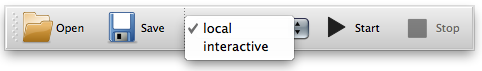
Execution mode: ''interactive'', ''local'' or ''remote''?
Simulations can be executed in different job queues for different tasks.
Local/interactive jobs are started in local job queue that is handled by Morpheus itself. Remote jobs are submitted over a ssh connection to the batch queuing system of the high performance computing resource (e.g. LSF).
Local / Interactive / Remote
Roughly, local mode is the 'normal' mode for simulation, while interactive mode is for rapid testing.
In interactive mode:
- Visual output (e.g. Gnuplotter) is directed to an on-screen terminal by overriding the specified terminal.
- Stop current interactive job from toolbar button.
Remote
Remote mode submits a job to the queueing system on a remote high performance computer.
Remote mode requires password-less ssh authentication (i.e. using ''ssh-copyid''). Specify username/password details under File → Preferences → Remote.
On first use, Morpheus copies a proxy script to the remote computer through which Morpheus communicates with the job scheduling system. Morpheus is shipped with a proxy script for LSF, but this can easily be adapted to other scheduling systems.
| Job queue | Purpose | Behavior |
|---|---|---|
| Local | Normal processing | |
| Remote | Remote batch processing | Submit job to remote queuing system (e.g. LSF) on high performance computing resource. Note: Feature not yet available in public version |
| Interactive | Testing mode | Start/Stop simulations from toolbar buttons. Directs visual output to on-screen terminal. Overrides Gnuplotter terminal to wxt (Linux), aqua (Mac) or win (Windows). |
FixBoard
When you open a outdated or broken XML model, Morpheus will try to automagically correct and update the model. For example, Morpheus creates required elements that are missing and removes obsolete elements.
The changes that Morpheus made are shown on the Fixboard. You are strongly advised to review those changes.
As an example, the following message will appear in the FixBoard when we invalidate the minimal model by removing the Description, Space and Time elements and replace them with an fictitious FakeNode node:
 <?xml version='1.0' encoding='UTF-8'?>
 <MorpheusModel version="1">
    <FakeNode/>
 </MorpheusModel>

FixBoard shows the automatic changes make in a broken or outdated model for review.
Note that this is a feature of graphical user interface. The command line interface morpheus cannot correct outdated or broken models supplied as command line arguments.
JobQueue
This panel has multiple functions:
- Overview of pending, running and terminated jobs
- Archive of simulation models
- Sorting simulation jobs and sweeps
- Access to simulation result browser
- Stop and remove jobs and results
Morpheus results browser
Simulation results can be shown by clicking the job in the JobQueue. This opens a file browser within Morpheus showing the Output Folder and the Output Text.
File browser and terminal
The buttons above the result browser can be used to open the Output Folder your system-wide file browser or open in a Terminal.
Output Folder in your file browser or in terminal.Change results folder
To change the folder where results are stored, check the Settings.
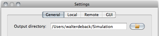
File→Settings.
Reset JobQueue archive
The information in the JobQueue is stored in using a SQLite database. This database is named morpheus.db.sqlite and stored in the OS-specific folder for Application Data.
Remove or rename the file morpheus.db.sqlite to reset the job archive. Note that this does not remove the simulation results themselves.
Checkpointing (simulation snapshots)
Checkpointing
Storing snapshots of the simulation state during execution is called checkpointing.
This allows the user to e.g.:
- Restore a simulation
- Continue a simulation under different conditions
- Use the end-state of a simulation as initial condition of a new simulation
Enable checkpointing
Checkpointing is switched off by default.
To enable checkpointing, add the item Time → SaveInterval.
To set the interval, set the Time → SaveInterval → value.
Special cases:
- value = -1: Disable checkpointing
- value = 0: Store state only at start and end
- value > 0: Store state at specified time interval
File format
Snapshots are saved in a compressed XML format with the filename [Title][Time].xml.gz.
Open saved models
Snapshot files [Title][Time].xml.gz can be opened by double-clicking on them in the GUI.
From the command line, first unzip the file and then run morpheus [Title][Time].xml
Limitations
The snapshots store the complete simulation state. However, the values of PDE Layers are not stored.
This is excluded because of (1) the large storage requirements and (2) the required time to write to text file. (In the future, separate binary files will be written for PDE Layeres which can be stored and written more efficiently, but are more difficult to do in a platform independemt fashion.)
Restore parameter sweeps
Parameter sweeps can also be restored. This restores the parameters and value ranges specified for a particular model.
This feature requires an opened model that has the same parameters.
Settings
Multithreading / Concurrent jobs
- Number of threads: Used to set number of openMP threads for (in-job parallelization)
- Concurrent jobs: number of jobs executed in parallel (between-job parallelization)
By default, Morpheus uses the first GnuPlot executable it can find in the PATH environmental variable. Optionally, you can overrule this path.
Graphical User Interface
To use a specific GnuPlot version, specify you gnuplot executable under File → Settings → Local → Gnuplot executable.
Command Line Interface
To specify a gnuplot executable from the command line, you can use the gnuplot-part option as command line argument:
morpheus -gnuplot-path [File]